DataStage

Extraction, Transformation & Loading

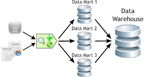
In computing, Extract, Transform and Load (ETL) refers to a process in database usage and especially in data warehousing that:

• Extracts data from homogeneous or heterogeneous data sources
• Transforms the data for storing it in the proper format or structure for the purposes of querying and analysis
• Loads it into the final target (database, more specifically, operational data store, data mart, or data warehouse)

Usually all the three phases execute in parallel since the data extraction takes time, so while the data is being pulled another transformation process executes, processing the already received data and prepares the data for loading and as soon as there is some data ready to be loaded into the target, the data loading kicks off without waiting for the completion of the previous phases.

ETL systems commonly integrate data from multiple applications (systems), typically developed and supported by different vendors or hosted on separate computer hardware. The disparate systems containing the original data are frequently managed and operated by different employees. For example, a cost accounting system may combine data from payroll, sales, and purchasing.

The ETL process consists of the following steps:

1. Initiation
2. Build reference data
3. Extract from sources
4. Validate
5. Transform
6. Load into stages tables
7. Audit reports
8. Publish
9. Archive
10. Clean up

How do the ETL tools work?

• The first task is data extraction from internal or external sources. After sending queries to the source system data may go indirectly to the database. However usually there is a need to monitor or gather more information and then go to Staging Area . Some tools extract only new or changed information automatically so we dont have to update it by our own. 
• The second task is transformation which is a broad category:  transforming data into a stucture wich is required to continue the operation (extracted data has usually a sructure typicall to the source) 

1. sorting data 
2. connecting or separating 
3. cleansing 
4. checking quality 

• The third task is loading into a data warehouse.

Comercial ETL Tools:

Informatica - Power Center

IBM - Websphere DataStage(Formerly known as Ascential DataStage)

SAP - BusinessObjects Data Integrator

IBM - Cognos Data Manager (Formerly known as Cognos DecisionStream)

Microsoft - SQL Server Integration Services

Oracle - Data Integrator (Formerly known as Sunopsis Data Conductor)

SAS - Data Integration Studio

Oracle - Warehouse Builder

Freeware, open source ETL tools:

Pentaho Data Integration (Kettle)

Talend Integrator Suite

CloverETL

Jasper ETL

DataStage  Introduction

IBM InfoSphere DataStage is an ETL Tool and it is client-server technology and integrated tool set used for designing, running, monitoring and administrating the “data acquisition” application is known as “job”.
IBM InfoSphere DataStage is an ETL tool and part of the IBM Information Platforms Solutions suite and IBM InfoSphere. It uses a graphical notation to construct data integration solutions and is available in various versions such as the Server Edition, the Enterprise Edition, and the MVS Edition.

In the year, 2005, it was under the acquisition of IBM. DataStage was added to the family of WebSphere. Then, from the year 2006, it officially came to be known as IBM WebSphere DataStage. The name was again changed in the year to IBM InfoSphere DataStage.

A job is graphical representation of data flow from source to target and it is designed with source definitions and target definition and transformation Rules. The data stage software consists of client and server components

PC is having 4 components These are the client components.

1.  DATA STAGE ADMINISTRATOR : This components will be used for to perform create or delete the projects. , cleaning metadata stored in repository and install NLS.
2.  DATA STAGE DESIGNER :  It is used to create the Datastage application known as job. The following activities can be performed with designer window.
   a) Create the source definition.
   b) Create the target definition.
   c) Develop Transformation Rules
   d) Design Jobs.
3.  DATA STAGE DIRECTOR :  It is used to validate, schedule, run and monitor the Data stage jobs.
4.  DATA STAGE MANAGER :  it will be used for to perform the following task like..
   a) Create the table definitions.
   b) Metadata back-up and recovery can be performed.
   c) Create the customized components.

Data Stage Repository:-It is one of the server side components which is defined to store the information about to build out Data Ware House.

Jobs:

job is nothing but it is ordered series of individual stages which are linked together to describe the flow of data from source and target. There are three types of jobs can be designed.

a) Server jobs
b) Parallel Jobs
c) Mainframe Jobs

Difference between server jobs and parallel jobs
1. Server jobs:-

•  In server jobs it handles less volume of data with more performance.
•  It is having less number of components.
•  Data processing will be slow.
•  It’s purely work on SMP (Symmetric Multi Processing).
•  It is highly impact usage of transformer stage.

2. Parallel jobs:-

•  It handles high volume of data.
•  It’s work on parallel processing concepts.
•  It applies parallelism techniques.
•  It follows MPP (Massively parallel Processing).
•  It is having more number of components compared to server jobs.
•  It’s work on orchestrate framework

1. SMP (symmetric multiprocessing)

• in which some hardware resources might be shared among processors. The processors communicate via shared memory and have a single operating system.
• Symmetric Multi-Processing. In a symmetrical multi-processing environment, the CPU's share the same memory,and as a result code running in one CPU can affect the memory used by another.

2. Cluster or MPP (massively parallel processing)

• also known as shared-nothing, in which each processor has exclusive access to hardware resources. MPP systems are physically housed in the same box, whereas cluster systems can be physically dispersed. The processors each have their own operating system, and communicate via a high-speed network.
• MPP: Massively Parallel Processing. computer system with many independent arithmetic units or entire microprocessors, that run in parallel.

Parallelism in Data Stage

• it is a process to perform ETL task in parallel approach need to build the data warehouse. The parallel jobs support the following hardware system like SMP, MPP to achieve the parallelism.

There are two types of parallel parallelism techniques.

1. Pipeline parallelism.:- the data flow continuously throughout it pipeline . All stages in the job are Operating simultaneously. For example, my source is having 4 records as soon as first record starts processing, then all remaining records processing simultaneously.
2. Partition parallelism:- in this parallelism, the same job would effectively be run simultaneously by several processors. Each processors handles separate subset of total records. For example, my source is having 100 records and 4 partitions. The data will be equally partition across 4 partitions that mean the partitions will get 25 records. Whenever the first partition starts, the remaining three partitions start processing simultaneously and parallel.

Configuration file
It is normal text file. it is having the information about the processing and storage resources .that are available for usage during parallel job execution.
The default configuration file is having like

1.  Node:- it is logical processing unit which performs all ETL operations.
2.  Pools:- it is a collections of nodes.
3.  Fast Name: it is server name. by using this name it was executed our ETL jobs.
4.  Resource disk:- its permanent memory area which stores all Repository components.
5.  Resource Scratch disk:-it is temporary memory area where the staging operation will be performed.

Partitioning Techniques

1. Partitioning mechanism divides a portion of data into smaller segments, which is then processed independently by each node in parallel. It helps make a benefit of parallel architectures like SMP, MPP, Grid computing and Clusters.
2. Collecting is the opposite of partitioning and can be defined as a process of bringing back data partitions into a single sequential stream (one data partition). 

Data partitioning methods

Datastage supports a few types of Data partitioning methods which can be implemented in parallel stages:

Auto(default) : Datastage Enterprise Edition decides between using Same or Round Robin partitioning. Typically Same partitioning is used between two parallel stages and round robin is used between a sequential and an EE stage.

Same : existing partitioning remains unchanged. No data is moved between nodes.

Round robin : rows are alternated evenly accross partitions. This partitioning method guarantees an exact load balance (the same number of rows processed) between nodes and is very fast.

Hash : rows with same key column (or multiple columns) go to the same partition. Hash is very often used and sometimes improves performance, however it is important to have in mind that hash partitioning does not guarantee load balance and misuse may lead to skew data and poor performance.

Entire : all rows from a dataset are distributed to each partition. Duplicated rows are stored and the data volume is significantly increased.

Random : rows are randomly distributed accross partitions.

Range : an expensive refinement to hash partitioning. It is imilar to hash but partition mapping is user-determined and partitions are ordered. Rows are distributed according to the values in one or more key fields, using a range map (the 'Write Range Map' stage needs to be used to create it). Range partitioning requires processing the data twice which makes it hard to find a reason for using it.

Modulus : data is partitioned on one specified numeric field by calculating modulus against number of partitions. Not used very often.

Data collecting methods

A collector combines partitions into a single sequential stream. Datastage EE supports the following collecting algorithms:

Auto : the default algorithm reads rows from a partition as soon as they are ready. This may lead to producing different row orders in different runs with identical data. The execution is non-deterministic.

Round Robin : picks rows from input partition patiently, for instance: first row from partition 0, next from partition 1, even if other partitions can produce rows faster than partition 1. 

Ordered : reads all rows from first partition, then second partition, then third and so on.

Sort Merge : produces a globally sorted sequential stream from within partition sorted rows. Sort Merge produces a non-deterministic on un-keyed columns sorted sequential stream using the following algorithm: always pick the partition that produces the row with the smallest key value.

Data Warehouse

Introduction

        Data ware house is a data base which maintains the data from different data sources. It is use to maintain the historical information.

•  A data warehouse is constructed by integrating data from multiple heterogeneous sources that support analytical reporting, structured or adhoc queries, and decision making. Data warehousing involves data cleaning, data integration, and data consolidations.

• In computing, a data warehouse also known as an enterprise data warehouse is a system used for reporting and data analysis. DWs are central repositories of integrated data from one or more disparate sources.

Founders of data ware house:-

1. Will Inman : The first DWH system is implemented in 1987 by Inman. According to will Inman DWH is a system which is ment for query and analyzing rather then the transactional process.
2.  Ralph Kimball:- Mentioned 4 characteristics on data ware house

• Time variant system:- DWH allows the users to analysis the data at different levels of times like years, Half-yearly,quarterly,weak,hour..Hence it is a time variant system.
• Non-volatile database:- The data is loaded from source system is static in nature and that is when the datab is loaded from source system to target system. The target data is not reflected by the changes that are made on the source
• subject oriented database:- The data ware house as a capability to maintain diff subject of data. Ex: sales, hr, loans.
• Integrated data base:- The data in the DWH system is integrated from d.H data source.  this all of the 4 types is called as characteristics futures of data ware house.

Why Data Warehousing?

• Improved user access: a standard database can be read and manipulated by programs like SQL Query Studio or the Oracle client, but there is considerable ramp up time for end users to effectively use these apps to get what they need. Business intelligence and data warehouse end user access tools are built specifically for the purposes data warehouses are used: analysis, bench marking, prediction and more.
• Better consistency of data: developers work with data warehousing systems after data has been received so that all the information contained in the data warehouse is standardized. Only uniform data can be used efficiently for successful comparisons. Other solutions simply cannot match a data warehouse's level of consistency.
• All-in-one: a data warehouse has the ability to receive data from many different sources, meaning any system in a business can contribute its data. Let's face it: different business segments use different applications. Only a proper data warehouse solution can receive data from all of them and give a business the "big picture" view that is needed to analyze the business, make plans, track competitors and more.
• Future-proof: a data warehouse doesn't care where it gets its data from. It can work with any raw information and developers can "massage" any data it may have trouble with. Considering this, you can see that a data warehouse will outlast other changes in the business' technology. For example, a business can overhaul its accounting system, choose a whole new CRM solution or change the applications it uses to gather statistics on the market and it won't matter at all to the data warehouse. Upgrading or overhauling apps anywhere in the enterprise will not require subsequent expenditures to change the data warehouse side..
• Advanced query processing: in most businesses, even the best database systems are bound to
  either a single server or a handful of servers in a cluster. A data warehouse is a purpose-built hardware solution far more advanced than standard database servers. What this means is a data warehouse will process queries much faster and more effectively, leading to efficiency and
  increased productivity.
• Retention of data history: end-user applications typically don't have the ability, not to mention the space, to maintain much transaction history and keep track of multiple changes to data. Data warehousing solutions have the ability to track all alterations to data, providing a reliable history of all changes, additions and deletions. With a data warehouse, the integrity of data is ensured.
• Disaster recovery implications: a data warehouse system offers a great deal of security when it comes to disaster recovery. Since data from disparate systems is all sent to a data warehouse, that data warehouse essentially acts as another information backup source. Considering the data warehouse will also be backed up, that's now four places where the same information will be stored: the original source, its backup, the data warehouse and its subsequent backup. This is unparalleled information security.

Architecture of Data Warehouse

• Different data warehousing systems have different structures. Some may have an ODS (operational data store), while some may have multiple data marts. Some may have a small number of data sources, while some may have dozens of data sources. 

• Data Source :This represents the different data sources that feed data into the data warehouse. The data source can be of any format -- plain text file, relational database, other types of database, Excel file, etc., can all act as a data source. Many different types of data can be a data source:

1. Operations -- such as sales data, HR data, product data, inventory data, marketing data, systems data.
2. Web server logs with user browsing data.
3. Internal market research data.
4. Third-party data, such as census data, demographics data, or survey data.All these data sources together form the Data Source Layer.

• ETL (Extract Transform Load) : This is where data gains its "intelligence", as logic is applied to transform the data from a transactional nature to an analytical nature. This layer is also where data cleansing happens. The ETL design phase is often the most time-consuming phase in a data warehousing project, and an ETL tool is often used in this layer.
• Staging Area :The Data Warehouse Staging Area is temporary location where data from source systems is copied. A staging area is mainly required in a Data Warehousing Architecture for timing reasons. In short, all required data must be available before data can be integrated into the Data Warehouse.

1.  Due to varying business cycles, data processing cycles, hardware and network resource limitations and geographical factors, it is not feasible to extract all the data from all Operational databases at exactly the same time.
2.  For example, it might be reasonable to extract sales data on a daily basis, however, daily extracts might not be suitable for financial data that requires a month-end reconciliation process.Similarly, it might be feasible to extract "customer" data from a database in Singapore at noon eastern standard time, but thisnwould not be feasible for "customer" data in a Chicago database.
3.  Data in the Data Warehouse can be either persistent (i.e. remains around for a long period) or transient (i.e. only remains around temporarily).Not all business require a Data Warehouse Staging Area. For many businesses it is feasible to use ETL to copy data directly from operational databases into the Data Warehouse

   Operational Data Store (ODS) :

   Some definitions of an ODS make it sound like a classical data warehouse, with periodic (batch) inputs from various operational sources into the ODS, except that the new inputs overwrite existing data.

   In a bank, for example, an ODS (by this definition) has, at any given time, one account balance for each checking account, courtesy of the checking account system, and one balance for each savings account, as provided by the savings account system.

   The various systems send the account balances periodically (such as at the end of each day), and an ODS user can then look in one place to see each bank customer’s complete profile (such as the customer’s basic information and balance information for each type of account).

• Data Mart : ETL (Extract Transform Load) jobs extract data from the Data Warehouse and populate one or more Data Marts for use by groups of decision makers in the organizations.The Data Marts can be Dimensional (Star Schemas) or relational, depending on how the information is to be used and what "front end" Data Warehousing Tools will be used to present the information.
• Each Data Mart can contain different combinations of tables, columns and rows from the Enterprise Data Warehouse. For example, a business unit or user group that doesn't require a lot of historical data might only need transactions from the current calendar year. The Personnel Department might need to see all details about employees, whereas data such as "salary" or "home address" might not be appropriate for a Data Mart that focuses on Sales.

Top down and Bottom Up approach:

• Top down is nothing but first data populated into DWH, and then populated into data marts which are proposed by Ralph Kimball.
• Bottom Up approach is nothing but first data populated into datamarts, then populated into DWH which proposed by Will Inman.

OLTP vs. OLAP
We can divide systems into transactional (OLTP) and analytical (OLAP). In general we can assume that OLTP systems provide source data to data warehouses, whereas OLAP systems help to analyze it.

• OLTP (On-line Transaction Processing) is characterized by a large number of short on-line transactions (INSERT, UPDATE, DELETE). The main emphasis for OLTP systems is put on very fast query processing, maintaining data integrity in multi-access environments and an effectiveness measured by number of transactions per second. In OLTP database there is detailed and current data, and schema used to store transactional databases is the entity model (usually 3NF).
• OLAP (On-line Analytical Processing) is characterized by relatively low volume of transactions. Queries are often very complex and involve aggregations. For OLAP systems a response time is an effectiveness measure. OLAP applications are widely used by Data Mining techniques. In OLAP database there is aggregated, historical data, stored in multi-dimensional schemas (usually star schema).

Fact table:
If a table contains more foreign keys and it gives summarized information such a table is called fact table.
The centralized table in a star schema is called ‘Fact table’ or The table which is having
measures and foreign keys of dimension tables as attributes(columns) is called Fact table. It

has a composite primary key with the foreign keys of Dimension table.
Factless Fact Table : A Fact table which doesn’t have measures or aggregates or facts called Factless Facttable.
Types of facts:
a)Aggregate: The facts which are having Aggregated values are called ‘Aggregative Facts’.
b)Non Aggregate:The facts which does not have Aggregated values are called ‘Non Aggregated Facts’.

Fact constellation:
 it is a measure of online analytical processing, which is a collection of multiple fact tables sharing dimension tables, viewed as a collection of stars. This is an improvement over Star schema.

Dimension table:
If a table contains primary keys and it gives detailed information about the table such table is called dimension table.

Confirm dimension:
A dimension table shared with more than one fact table in the schema then that table is called confirmed dimension.
Degenerated Dimension:
A fact table some times act as a dimension and it maintains relationship with another fact table such a table called Degenerated Dimension
Junk Dimension:
A dimension contains junk values like flags(0,1),genders(m,f),text values etc and which table not useful to generate reports is called Junk Dimension.
Dirty Dimension:
If a record maintains more than one time in a particular table by the reference Non key attribute such a table is called dirty dimension.

Data modeler can maintain two types of modelings in DWH.

1. Relational Modeling:  It is nothing but the entities are designed, in this model all tables are entities, never called Fact and dimension tables. This model may be second normal form or third normal form or in between 2nd and 3rd normal form.
   Entity:It can be anything in the real world, which has got certain properties, which is
   identifier through it. Entity can be a person or location or event or thing or corporation
   or which the database system stores the information. The characteristic of entity known as attribute. Each attribute represents one kind of property.
2. Dimensional Modeling: It is nothing but the data modeler design database in dimension tables and fact tables.

The dimension modeling can be classified again into 3 sub modelings.

• Star Schema Design:- A fact table surrounded by dimensions is called star schema. It looks like a star. In a star schema is there is only one table then it is called simple star schema. More than one Fact table available then it is called Complex star schema.
  
  
  
  
  
• Snow Flake Schema Design:
  When any one of the demoralized dimensional table is converted into the normalized table, then that structure is called "Snow Flake Schema Design"
  Advantage: It fallows the normalized structure it eliminates data Redundancy.
  Disadvantage: It degrades the performance level
  ( Note: Combination of Star Schema and Snow Flake Schema is called Multi
  Star Schema )
• 

Difference between star schema and snowflake schema: